
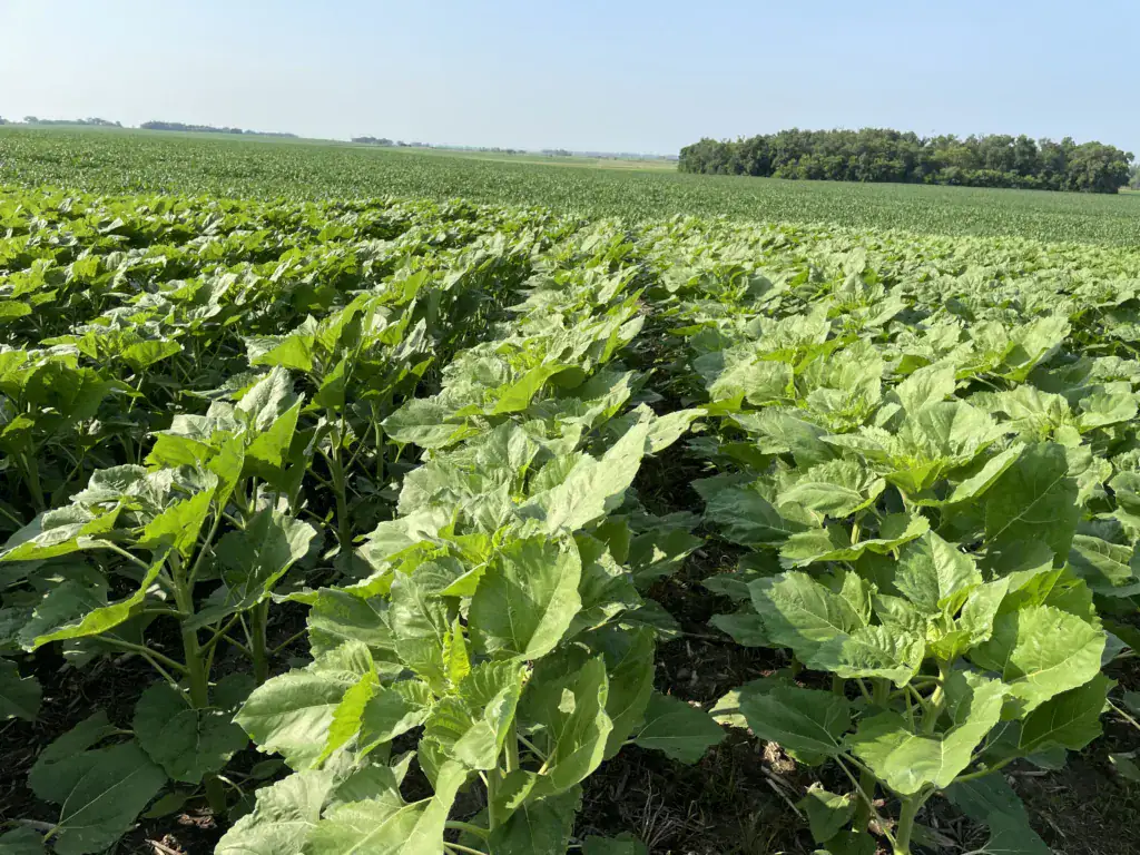
The AGRISTATLAB’s Split-Plot Design Generator is a specialized tool for researchers and plant breeders to create randomized split-plot field layouts for Plant breeding trials. Enter your main-plot factor, your subplot factor and the number of blocks, and the tool builds a randomized layout, a ready-to-use fieldbook, and an ANOVA skeleton that shows how the design should be analyzed. Before you use it, this post explains why and when to choose a split-plot design, and the statistical model behind it. You can read about other experimental designs, and when to use which one, in our blog on Understanding Experimental Designs. If you want to create a trial in RCBD, CRD or Alpha Lattice design, please use our Experimental Design Generator or Partially Replicated Design (pRep design).
What Is a Split-Plot Design?
A split-plot design is a factorial experiment in which the two factors are applied to experimental units of different sizes. The levels of the first factor (factor A, the main-plot factor) are assigned to large experimental units called main plots (also called whole plots). Each main plot is then divided into smaller subplots, and the levels of the second factor (factor B, the subplot factor) are assigned to the subplots within every main plot.
Randomization happens in two stages. First, the levels of A are randomly assigned to the main plots within each block. Second, the levels of B are randomly and independently assigned to the subplots within each main plot. Because there are two sizes of experimental unit, there are also two experimental errors: one for the main plots and one for the subplots. This is the key idea to remember, and it is what separates a split-plot from an ordinary two-factor RCBD.
Why Use a Split-Plot Design?
- Some factors are hard or expensive to change: Irrigation regimes, tillage systems, seeding dates, planting methods and fertilizer applications made with large equipment need big plots. Small plots would create interference between neighbouring treatments and are often impractical. Growth chambers and greenhouse benches create the same problem, since a temperature setting applies to everything inside.
- Different factors need different plot sizes: Varieties or breeding lines can be grown on small plots, while management practices need large ones. A split-plot lets you combine both in a single experiment.
- Higher precision where it matters: The subplot factor and the A × B interaction are compared within main plots, so they are usually estimated more precisely than in a comparable RCBD. The price is lower precision for the main-plot factor.
- Efficient use of land and resources: One set of large plots carries many subplot treatments, so you avoid repeating the large-plot treatment for every treatment combination.
- Interactions are the main interest: Questions such as “Does the ranking of varieties change under different seeding dates?” are exactly what a split-plot is built to answer.
The Statistical Model
For a split-plot design with the main plots arranged in a randomized complete block design (RCBD), the standard model is:
Yijk = μ + ρi + αj + δij + βk + (αβ)jk + εijk
- μ is the overall mean and ρi is the effect of block i (i = 1, …, r). Blocks are usually treated as random.
- αj is the effect of level j of the main-plot factor A (j = 1, …, a).
- δij is the main-plot (whole-plot) error, assumed independent with mean 0 and variance σδ2. It is the Block × A interaction.
- βk is the effect of level k of the subplot factor B (k = 1, …, b), and (αβ)jk is the A × B interaction.
- εijk is the subplot error, assumed independent with mean 0 and variance σε2.
The two error terms give the split-plot ANOVA its characteristic structure. The main-plot factor is tested against the main-plot error, while the subplot factor and the interaction are tested against the subplot error:
| Source of variation | df | Tested against |
|---|---|---|
| Block | r − 1 | — |
| A (main-plot factor) | a − 1 | Error(a) |
| Error(a) = Block × A | (r − 1)(a − 1) | — |
| B (subplot factor) | b − 1 | Error(b) |
| A × B | (a − 1)(b − 1) | Error(b) |
| Error(b) | a(r − 1)(b − 1) | — |
| Total | rab − 1 |
Comparisons between two main-plot means use Error(a), and comparisons between two subplot means within the same main plot use Error(b). Comparing A means at the same or different levels of B needs a weighted combination of the two error terms, which mixed-model software handles for you. Ignoring the two-error structure and analyzing the data as a simple two-way ANOVA is a common mistake. It makes the main-plot factor look more significant than it really is.
Which Factor Should Go on the Main Plot?
- Put the factor that needs large plots or is hard to change on the main plots.
- Put the factor you want to estimate most precisely (and its interaction with the other factor) on the subplots.
- If neither factor is constrained, put the factor where you expect larger differences on the main plots, because lower precision is acceptable there.
Planning Your Design: Points to Watch
- Degrees of freedom for Error(a): With few main-plot levels and few blocks, Error(a) can have very few degrees of freedom, so the test of the main-plot factor has low power. With 2 main-plot levels and 4 blocks, Error(a) has only 3 df. If the main-plot factor matters, add blocks or locations.
- Use at least two blocks: Without replication of the main plots there is no Error(a) at all.
- Randomize both stages: Main-plot levels are randomized within each block, and subplot levels are randomized separately within each main plot. The generator below does both.
- Not the same as repeated measures: If the “subplot” factor is time or depth, it cannot be randomized, and the analysis needs a different covariance structure.
- Missing subplots are manageable, missing main plots are costly: Losing an entire main plot removes all of its subplots and unbalances the main-plot comparisons.
Key Features of the Split-Plot Design Generator
- Flexible Factor Setup
- Name your own main-plot and subplot factors and list their levels
- Any number of blocks (two or more)
- Choose how many main plots sit side by side in each field row
- Two-Stage Randomization
- Main-plot levels randomized within each block, subplot levels randomized within each main plot
- Seed-controlled randomization for reproducible designs
- One-click re-randomization
- Multi-Location Trial Support
- Design trials for several locations at once, each with its own randomization
- Consolidated fieldbook with location metadata
- Clear Field Layout
- Agricultural-standard coordinate system (1,1 = bottom-left corner)
- Main plots outlined and color-coded, with subplot treatments labelled inside
- Live design summary with degrees of freedom and warnings
- Comprehensive Outputs
- Download the field layout as a PNG image
- Export the complete fieldbook as CSV (compatible with R, SAS, etc.)
- ANOVA skeleton and starter R code that match your design
How It Works
- Enter the trial name and the location(s)
- Define the main-plot factor and the subplot factor, with their levels separated by commas
- Set the number of blocks and, if you like, how many main plots go in each field row
- Generate the randomized design, and re-randomize if you want a different draw
- Review the layout, fieldbook and ANOVA skeleton
- Download the fieldbook and the layout map
Worked Example
The tool below is pre-filled with a typical example: three seeding dates (main-plot factor: Early, Medium, Late) crossed with six varieties (subplot factor: V1 to V6) in four blocks. Each block contains 3 main plots, and each main plot is split into 6 subplots, so the trial has 12 main plots and 72 plots per location. The degrees of freedom are Block 3, Seeding date 2, Error(a) 6, Variety 5, Seeding date × Variety 10 and Error(b) 45, for a total of 71. Try changing the number of blocks and watch how Error(a) changes.
Split-Plot Experimental Design Generator
Create a randomized split-plot layout with a main-plot factor and a subplot factor, arranged in blocks (RCBD).
1. Trial Information
2. Main-Plot Factor
Assigned to the large plots. Randomized within each block.
3. Subplot Factor
Assigned to the small plots inside every main plot. Randomized within each main plot.
4. Blocks and Field Layout
Each block fills one or more field rows. Use a smaller number to make a narrower field.
Design Output
Thick outlines mark main plots. Each cell shows the main-plot level (small), the subplot level (bold) and the (row, column) position. Row 1, column 1 is the bottom-left corner.
The skeleton applies to each location analyzed separately. For a combined analysis across locations, add location terms to the model.
Starter R code
Further Reading
- Gomez, K.A. and Gomez, A.A. Statistical Procedures for Agricultural Research. Wiley.
- Federer, W.T. and King, F. Variations on Split Plot and Split Block Experiment Designs. Wiley.
- Montgomery, D.C. Design and Analysis of Experiments. Wiley.
This tool streamlines the process of designing a split-plot experiment, replacing manual randomization and spreadsheet planning with an automated, statistically valid approach tailored for agricultural research. Your feedback is very important for us. Please drop your feedback here.